Graph-based Representation of Arbitrary Binary Linear Codes: A Novel Algorithmic Approach

Olufemi Ololade Olaewe; Peter Awonnatemi Agbedemnab; Moses Apambila Agebure

doi:doi:10.11648/j.mcs.20261102.12

Research Article |

| Peer-Reviewed

Graph-based Representation of Arbitrary Binary Linear Codes: A Novel Algorithmic Approach

Olufemi Ololade Olaewe^*

, Peter Awonnatemi Agbedemnab

, Moses Apambila Agebure

Published in Mathematics and Computer Science (Volume 11, Issue 2)

Received: 21 April 2026 Accepted: 30 April 2026 Published: 12 May 2026

Views: Downloads:

Download PDF

Share This Article

Twitter
Linked In
Facebook

Abstract

This study presents a novel algorithm for transforming binary linear codes with parameters (n,k,d) into a bipartite graph representation. The proposed method explicitly represents each codeword as a node, enabling a complete structural visualization of the code. The algorithm is implemented and its computational performance is analyzed, demonstrating linear complexity with respect to code length (n) and exponential complexity with respect to dimension (k). The correctness and interpretability of the approach are illustrated using representative examples of (4,2) and (6,3) linear codes, where the resulting graphical structures reveal clear and meaningful patterns. In addition, the proposed representation is shown to be information-complete and to preserve code equivalence through graph isomorphism. The representation is particularly well-suited for integration with modern graph-based machine learning techniques, such as Graph Neural Networks, where structural information plays a central role in learning. Furthermore, the scalability characteristics of the algorithm make it applicable to a wide range of code parameters, while maintaining consistency in representation. To further assess the effectiveness of the proposed algorithm, it is compared with existing methodologies, including Trellis and Tanner graph representations, demonstrating advantages in structural analysis, effectiveness for graph-based learning, and its unique representation of the zero codeword. This framework therefore serves as a foundation for structural analysis of linear codes, facilitates equivalence testing, and is naturally suited for integration with graph-based machine learning models.

Published in	Mathematics and Computer Science (Volume 11, Issue 2)
DOI	10.11648/j.mcs.20261102.12
Page(s)	33-44
Creative Commons	This is an Open Access article, distributed under the terms of the Creative Commons Attribution 4.0 International License (http://creativecommons.org/licenses/by/4.0/), which permits unrestricted use, distribution and reproduction in any medium or format, provided the original work is properly cited.
Copyright	Copyright © The Author(s), 2026. Published by Science Publishing Group

Keywords

Linear Code Equivalence, Linear Code, Graph Theory, Algorithm

1. Introduction

Linear codes are essential tools in coding theory, with vast applications in error correction, communication systems, and cryptography. A linear code is typically denoted by [n, k, d] with n being the length, k indicates the dimension, and d denotes the minimum Hamming distance. These codes also play a crucial role in post-quantum cryptography systems, such as McEliece cryptosystem.

A closely related concept is linear code equivalence which states that two codes say A and B, can be considered equivalent if and only if A can be transformed by permuting coordinate positions or with operations such as column scaling. Linear code equivalence computation gained recognition in literature as it aids multiple representations of a code while maintaining properties, it is also useful in code classification and cryptanalysis

[1]

Tanner graph can be described as a bipartite graph to represent parity check matrix in graphical form. The graph uses variable nodes corresponding to codewords bits and check node corresponds to parity check constraint, also in this graphical representation, an edge is created between variable node and check node if and only if the bit participates in parity check equation

[2]

. Tanner graph was mainly used to aid decoding algorithms and was used for message transmission concepts such as belief propagation (BP) algorithm. Tanner graph was proposed originally to construct long codes from smaller ones, but later

[3]

used the concept as a foundation to Low Density Parity Check Code (LDPC).

BP algorithm can efficiently decode Low Density Parity Check Code (LDPC) by passing messages along the edges of Tanner graph. In definition, LDPC are represented by sparse parity-check matrices and are further represented using Tanner graph (TG) in order to aid Shanon-limit performance with manageable performance complexity

[5]

It is crucial to note that researchers use summarized representations i.e. generator and parity-check matrices that define the code. To the best of our knowledge, existing graph-based methodologies representing linear codes primarily focus on parity constraints and each codeword is not explicitly model as a node within the graph structure. This limitation restricts their applicability in tasks that require a complete structural view of the code, such as equivalence testing and learning-based analysis.

Graphical representations of linear codes have a rich history. With decoding as a yardstick, Tanner (1981) proposed the use of bipartite graphs to represent linear block codes using their parity-check matrices. The researcher opined that the graphical representation would provide a visual mapping of the bits which participate in each parity check.

The framework proposed by

[2]

has been the foundation of LDPC codes as noted by

[3]

and others. Variants of Tanner graphs and related graphical models have been applied to decoding, code construction, and code analysis. As a result of the proposition of various graph models, important properties such as girth, cycles which impact decoder performance are made available. Despite the prevalence of the Tanner graph for decoding, little literature exists on graphical representations that capture all codewords of a code.

While Tanner graphs and related representations have been widely used for decoding and constraint-based analysis, they do not provide a complete representation of the codeword space. In particular, the absence of explicit codeword-level representation limits their effectiveness in problems where global structural properties are essential. This motivates the need for a representation that captures the full set of codewords within a unified graphical framework.

To address this limitation, we introduce a novel bipartite graph representation of binary linear codes in which one partition corresponds to bit positions and the other corresponds to individual codewords. Unlike traditional representations, the proposed approach explicitly encodes the full codeword set, enabling complete structural characterization. Furthermore, we establish that this representation is information-complete and that linear code equivalence under coordinate permutation corresponds directly to graph isomorphism under the proposed construction.

1.1. Linear Codes and Tanner Graphs

Traditionally, the representation of linear codes is done algebraically. Linear code can be represented using Generator matrix G (k × n) that spans the code or by parity-check matrix H ((n − k) × n) that depicts code’s constraints.

Tanner proposed a graphical measure to represent the parity-check structure of linear codes. In the graph representation, each check node enforces a parity-check equation and connect variable nodes (bits) that participate in the equation

[2]

Tanner graph became notable with LDPC codes where it is sparse, LDPC codes have relatively low average node degree and this is a crucial factor for the success of iterative decoders

[4]

. In the case where parity-check matrices are dense, its Tanner graph representation will equally have high degree nodes.

It is important to note that dense nodes are less useful for iterative decoding, this fact suggests why LDPC codes have received much attention in communication system. Outside LDPC and related sparse codes, Tanner graphs have not been leveraged in traditional coding theory analysis.

Research has leverage graph based representational for other purposes; for example graph model of codes has been used in graph neural network decoder, in this instance a neural network was trained on a Tanner graph to decode errors

[5]

demonstrated that dense code graphs can be processed using machine learning algorithms, the only limitation to this revelation is that limited work exist on constructing graphs for any linear code.

1.2. Graph-based Representation of Codes

The ability to carry out decoding on Tanner graph stems from the local nature of check constraints in the parity check. If a linear code TG is cycle-free, the maximum-likelihood decoding can be done in O(n²) time using dynamic programming

[6]

. Literature on coding theory has largely centered on algebraic invariants rather than graphical interpretation of general codes

[7]

TG bridged this knowledge gap for specific families i.e. LDPC and Turbo codes where the researcher indicated that these codes can in principle be represented as a graph using its parity check matrix. Parity check matrix for a (n,k,d) code can be graphically represented using a n×(n−k) bipartite graph where n columns correspond to bit nodes while n − k row correspond to check nodes

[8]

Another major evolution of Tanner graph is the expander codes which are constructed from bipartite expander graphs, in this case the graph structure directly influences code properties. It is crucial to note that expander graphs are sparse (a feature indicating prominence in decoding) but highly connected and has wide application in different areas including complexity theory, coding theory, algorithm design, cryptography, etc.

To the best of our knowledge, existing graphically representation of linear codes do not explicitly model all codewords within a unified bipartite structure and this can be attributed to the fact that most linear codes do not naturally have low density and hence will have a dense parity-check matrix (H) which will in turn not encourage its conversion to graph. Linear code without low density H would have O(n²) edges. This worst-case quadratic complexity is not a fundamental barrier as graphs with thousands of nodes can have millions of edges which are still manageable for computer algorithms

[9]

1.3. Trellis Representations and Trellis-based Decoding

Other than Tanner graph, linear code can be represented by trellises-time-index graphical models. These graphs depict how codewords evolve through states. A trellis diagram is basically a state machine unrolling of a code: each path through trellis corresponds to a codeword.

Trellis diagrams have been used to represent convolutional codes, and some types of block code due to its ability to aid maximum-likelihood decoding via Viterbi algorithm. It is worth noting that only linear block code can be represented using a trellis diagram however its complexity is not always manageable.

States in trellis encapsulate past input history or parity context and are indicated as nodes at each time step in the diagram, also edges represent transitions labelled by bits. For optimal decoding of short codes or convolutional codes, trellis representation can be leveraged on. The Viterbi algorithm operates on trellis to find the codeword path with maximum likelihood.

In recent years, trellis representation was applied to Polar codes and related constructions. Polar codes are mainly decoded by successive cancellations. However, in

[10]

study, the researcher merges convolutional precoding with polar coding, and this led to the creation of trellis representation of convolutional code preceding the polar transform.

The result of

[10]

’s research is a concatenated code that is decodable using a sequential algorithm operating on a combined trellis/tree structure. PAC codes were reported to dramatically improve the finite-length performance of polar codes.

[10]

study is a striking example of how adding trellis-based component to a code can yield gains.

Summarily, trellis diagram offers a graph-based view in the time dimension and are essential tool for optimal decoding of certain codes via Viterbi. Recent literature like PAC codes do suggest that trellises are still relevant.

1.4. Small Dimension Binary Codes in Cryptography and Machine Learning

In research conducted by

[11]

, the researchers proposed the use of LDPC codes as compressed domain encoding for images, the researchers further revealed that neural network is able to classify images from LDPC encoded data with smaller models and higher accuracy than with arithmetic coding.

Also, recent literature revealed that structured binary codes including LDPC codes is able to encode information in ways that deep learning models can exploit effectively and hence yielding efficient models for classification task

[11, 12]

In all the highlighted cases, the dimensions of referenced codes are kept modest to enable full code analysis while the length can be large without fundamentally harming these applications.

Recent studies have opined that when full codeword enumeration or complete analysis is the goal, the complexity grows mainly with 2^k(number of codewords) and not with n i.e. length, also exhaustive search over all codewords becomes feasible only if k is small

[13, 14]

Summarily, increasing length n solely does not create an exponential bottleneck, only dimension k drives complexity. As a result of this many recent studies exploit very long codes (large n) with moderate k, since this approach enables structural code analysis to be done exhaustively while benefiting from long code properties like high distance.

In a study by

[15]

, exhaustive classification of all binary length 14 was achieved using graph-based equivalence method. Such results are possible because in those cases dimension k is small enough to enumerate all codewords for each code, this further confirms that small k linear codes are well suited to tasks like structural code analysis, visualization, and machine learning

[11, 13, 14]

It is critical to indicate that the exponential dependence on the dimension (k) is inherent to any scheme that requires explicit enumeration of all codewords. In practice, many applications in code analysis, classification, and machine learning focus on moderate values of (k), where full enumeration remains computationally feasible. This aligns with existing studies that exploit small-dimensional codes for exhaustive structural analysis.

2. Materials and Methods

2.1. Parity Check Based Approach to Generate Tanner Graph

The existing scheme to generate Tanner graph is the parity-check based approach, which was proposed by

[2]

Input: Parity-check matrix H of size (n − k) × n

Output: Tanner graph G = (V,E) with bit-nodes and check-nodes

Initialize n bit-nodes: B = {b₁,b₂,...,b_n}

Initialize n − k check-nodes: C = {c₁,c₂,...,c_n₋_k}

Initialize empty edge set: E = ∅ For each i = 1 to n − k:

– For each j = 1 to n:

If H [i,j] = 1, add edge e = (b_j,c_i) to E

Return graph G = (B ∪ C,E)

2.2. Gilbert–Varshamov Bound

To determine if the generated linear codes exist, the Gilbert–Varshamov bound as implemented by Hoffman et al. (1991) was used in this study.

Theorem: There exists a linear code of length n, dimension k, and distance d if

\sum_{i = 0}^{d - 2} (\binom{n - 1}{i}) < 2^{n - k}

(1)

Corollary: If n ̸= 1, d ̸= 1, then there exists an (n,k,d) linear code with

|C| \geq \frac{2^{n - 1}}{\sum_{i = 0}^{d - 2} (\binom{n - 1}{i})}

(2)

The corollary provides a lower bound for the number of codewords in a linear code of length n and distance d.

2.3. Python-based Implementation

To implement the proposed algorithm, Python programming language was chosen. Python’s acceptance in scientific computing, along with its comprehensive ecosystem for graph-based data processing make it suitable for this study. Comprehensive libraries such as NumPy for matrix operations, NetworkX which aid graph construction and manipulation, and Matplotlib for data visualization are made available by Python. All of which are essential in this research.

Furthermore, Python Environment enables seamless operation with machine learning concepts especially with frameworks such as PyTorch and TensorFlow.

3. Results and Discussions

In this section, We provide the algorithm to represent linear code in bipartite graphical form. Next, we illustrate the algorithm with examples, showing the Tanner graph for different codes and discussing their structural features.

3.1. Proposed Algorithm

Algorithm 1: Linear Code to Bipartite Graph Conversion

Require:

C = \{c^{1}, c^{2}, . . ., c^{|C|}\} \subseteq F^{2} ⁿ

, a binary linear code

Ensure:

G = (U ∪ V, E), a bipartite graph representation of C

1. U ← {p₁, p₂,..., p_n} (position nodes)

2. V ← {w₁, w₂,..., w_|C|} (codeword nodes)

3. E ← ∅

4. For j = 1 to |C| do

5. Let

c^{j} = (c^{1 (j)}, c^{2 (j)}, . . ., c ₙ^{j})

6. For i = 1 to n do

7. If

c ᵢ^{j}

= 1 then

8. Add edge (pᵢ, w_j) to E

9. End If

10. End For

11. End For

12. Return G = (U ∪ V, E)

3.2. Runtime Behavior of the Proposed Algorithm

To evaluate the practical feasibility of the proposed scheme, Runtime analysis was conducted using linear codes with different parameters [n,k,d]. This was done to observe how the runtime changes as a function of:

Code length (n)

Code dimension (k): this determines the total number of codewords |C| = 2^k.

3.2.1. Setup and Measurement

Using a mid-range workstation (AMD Intel i7 processor with 16 GB RAM), the algorithm was implemented using Python programming language. Standard timing utilities were included in the implementation such that average time-taken to construct graphical representations of the linear codes are recorded.

Table 1. Observed runtime on different parameter [n,k].

Code Dimension k	Code Length n	Codewords 2^k	Edges	Average Runtime(ms)
4	10	16	80	2
6	20	64	512	5
8	30	256	2,880	18
10	50	1,024	20,480	55
12	50	4,096	204,800	210
14	50	16,384	819,200	960

To establish runtime growth rate, the proposed algorithm was evaluated using increasing linear code dimensions whiles maintaining moderate code lengths. Recorded results consistently indicate a predictable exponential growth both in edge count and runtime, this behaviour further confirms the theoretical complexity

(O (n \cdot 2^{k})) .

However, despite this growth rate, the implementation remains efficient for moderate dimensions, and hence supporting its applicability in practical scenarios involving structural code analysis.

3.2.2. Observations

Linear growth of the runtime is observed in relation to the length n, this is consistent with the algorithm’s time complexity of O(n · 2^k).

In terms of the dimension k, exponential growth of runtime is observed i.e increment in dimension k doubles the number of codewords as well as significant increase in the number of graph edge.

Beyond runtime performance, it is important to examine the structural growth of the resulting graph. The number of nodes in the proposed representation grows as (n + 2^k), while the number of edges grows as

(O (n \cdot 2^{k})) .

This reflects the explicit representation of all codewords, which distinguishes the proposed method from traditional parity-check-based graphs that scale primarily with (n) and (n-k).

This structural expansion is not a limitation but a direct consequence of explicitly representing the full codeword space. Consequently, the representation is particularly suitable for applications such as code equivalence testing and graph-based learning, where full structural information is required.

3.2.3. Practical Implication

The results affirm the efficiency of the algorithm; it can be established that increasing the length n of linear codes does not lead to performance bottleneck. Furthermore, the results obtained suggest completeness of the algorithm and therefore uphold its application in code structure analysis, visualization, and machine learning where completeness is more critical than real time speed.

3.3. Theoretical Properties of the Proposed Representation

The proposed algorithm is not only a visualization tool but also possesses essential theoretical properties. In particular, it is information-complete and preserves equivalence structure, as formalized below.

3.3.1. Theorem 1: Information-completeness of the Representation

Let

C \subseteq F_{2}^{n}

be a binary linear code and let

G_{C} = (U, V, E)

be the bipartite graph constructed using the proposed algorithm, where

U

represents bit-position nodes and

V

represents codeword nodes.

Then, the graph

G_{C}

uniquely determines the code

C

. That is, there exists a one-to-one correspondence between

C

and

G_{C}

Proof

Let

C = {c^{(1)}, c^{(2)}, \dots, c^{(m)}} \subseteq F_{2}^{n}

, where

m = ∣ C ∣

, and let the corresponding bipartite graph be

G_{C} = (U \cup V, E)

with:

U = \{p_{1}, p_{2}, \dots, p_{n}\}, V = \{w_{1}, w_{2}, \dots, w_{m}\} .

Define the edge set:

E = \{(p_{i}, w_{j}) \in U \times V : c_{i}^{\{(j)\}} = 1\} .

For each

w_{j} \in V

, define its neighborhood:

N (w_{j}) = \{p_{i} \in U : (p_{i}, w_{j}) \in E\} .

By construction, we have:

N (w_{j}) = \{p_{i} \in U : c_{i}^{\{(j)\}} = 1\}

which implies that the neighborhood

N (w_{j})

uniquely determines the support of the codeword

c^{(j)}

, i.e.,

supp (c^{j}) = \{i \in \{1, \dots, n\} : p_{i} \in N (w_{j})\} .

Therefore, each codeword

c^{(j)} \in C

can be uniquely reconstructed from the adjacency structure of

w_{j}

Define the mapping:

ϕ : V \to C, ϕ (w_{j}) = c^{(j)} .

From the construction,

ϕ

is well-defined and injective, since distinct nodes

w_{j} \neq w_{k}

correspond to distinct neighborhoods and hence distinct codewords.

Moreover,

ϕ

is surjective by definition of

V

, as every codeword in

C

is represented by some node in

V

Hence,

ϕ

is bijective.

Consequently, the graph

G_{C}

encodes all information necessary to reconstruct

C

, and the mapping between

C

and

G_{C}

is one-to-one.

3.3.2. Theorem 2: Code Equivalence and Graph Isomorphism

Let

C_{1}, C_{2} \subseteq F_{2}^{n}

be binary linear codes, and let

G_{C_{1}} = (U_{1} \cup V_{1}, E_{1}), G_{C_{2}} = (U_{2} \cup V_{2}, E_{2})

be their corresponding bipartite graph representations.

Then:

C_{1} \sim C_{2} ⟺ G_{C_{1}} ≅ G_{C_{2}},

where equivalence is under coordinate permutation and graph isomorphism preserves the bipartition.

Proof

Let

C_{1} = {c^{(1)}, \dots, c^{(m)}}, C_{2} = {d^{(1)}, \dots, d^{(m)}} .

Their graph representations are defined as

G_{C_{1}} = (U_{1} \cup V_{1}, E_{1}), G_{C_{2}} = (U_{2} \cup V_{2}, E_{2}),

where

E_{1} = {(p_{i}, w_{j}) : c_{i}^{(j)} = 1}, E_{2} = {(q_{i}, z_{j}) : d_{i}^{(j)} = 1} .

(

\Rightarrow

) Suppose

C_{1} \sim C_{2}

Then there exists a permutation

π \in S_{n}

such that

C_{2} = {π (c) : c \in C_{1}} .

Define

φ (p_{i}) = q_{π (i)}, φ (w_{j}) = z_{j^{'}},

where

d^{(j^{'})} = π (c^{(j)})

(p_{i}, w_{j}) \in E_{1}

, then

c_{i}^{(j)} = 1

, hence

d_{π (i)}^{(j^{'})} = 1

, implying

(q_{π (i)}, z_{j^{'}}) \in E_{2} .

Thus,

φ

preserves adjacency and is an isomorphism.

(

\Leftarrow

) Suppose

G_{C_{1}} ≅ G_{C_{2}}

. Then there exists a bijection

φ

preserving adjacency and bipartition, inducing a permutation

π \in S_{n}

such that

φ (p_{i}) = q_{π (i)} .

For any

w_{j}

, let

φ (w_{j}) = z_{j^{'}}

Then adjacency preservation implies

c_{i}^{(j)} = d_{π (i)}^{(j^{'})} \forall i,

d^{(j^{'})} = π (c^{(j)}) .

Hence,

C_{2} = {π (c) : c \in C_{1}},

and therefore

C_{1} \sim C_{2}

3.4. Illustrative Example of Graph Construction

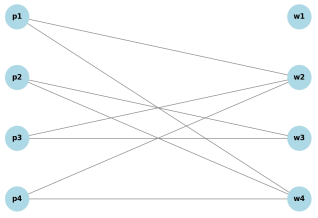
To demonstrate the proposed algorithm, it is applied to a simple linear code with parameters (4,2).

C = {0000, 1011, 0110, 1101}

The above code has length n = 4, dimension k = 2, and contains 2^k= 4 codewords.

Using the proposed algorithm, a bipartite graph is generated with:

4 bit-position nodes: p₁, p₂, p₃, p₄

4 codeword nodes: w₁, w₂, w₃, w₄

Edges representing 1s in each codeword at corresponding bit positions.

The output graph is thus Figure 1. Each of the edge in the graph connects a codeword node to the position node if and only if it has a value of 1. For instance, the second codeword 1011 (i.e w₂) is connected to positions p₁, p₃, and p₄, reflecting the 1s in the first, third, and fourth positions of the codeword.

Download: Download full-size image

Figure 1. Bipartite graph constructed from the codewords {0000, 1011, 0110, 1101}.

Left nodes are the bit positions (p₁to p₄) while the right nodes are the codewords (w₁to w₄) in the linear code. Edges reflect occurrence of 1 in codeword-bit position pairs.

The proposed algorithm is able to generate graphical representation of the linear code in this instance in approximately 0.11 milliseconds, this further confirms its efficiency even at small scales. This illustration validates that the algorithm correctly convert the linear code into an interpretable bipartite graph form, providing a solid foundation for further analysis such as equivalence testing and graph-based learning.

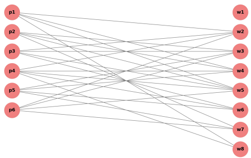
3.5. Illustrative Example of Bipartite Graph Construction (Complex Case)

To measure the efficiency of the proposed algorithm, it is applied to a linear code with higher length and dimension. In this instance a linear code with parameters (6,3) is used.

C = {000000, 101101, 011011, 110110, 111101, 001110, 010011, 100100}

This code has length n = 6, dimension k = 3, and contains 2^k= 8 codewords. Using the algorithm described in Section 6.3, a bipartite graph was constructed with:

6 bit-position nodes: p₁, p₂, p₃, p₄, p₅, p₆

8 codeword nodes: w₁to w₈

Edges representing 1s in each codeword at the corresponding bit positions.

The resulting graph is shown in Figure 2. Each edge connects a codeword node to the bit positions where it has a value of 1. For example, codeword 101101 (node w₂) is connected to positions p₁, p₃, p₄, and p₆, reflecting the 1s in those respective positions.

Download: Download full-size image

Figure 2. Bipartite graph constructed from a (6,3) binary linear code.

Bit position nodes (p₁to p₆) appear on the left, and codeword nodes (w₁to w₈) on the right. Edges connect codeword nodes to bit positions where they have 1s. The graph construction was achieved in approximately 0.35 milliseconds, indicating computational efficiency of the scheme at moderate dimensions. This further confirms that the proposed algorithm accurately scales to larger linear coeds with interpretability of the resulting graph being preserved. The output graphical representation explicitly shows the bit positions which are involved in participating codewords, enabling visual inspection and offering solid basis for tasks such as code equivalence testing and graph-based machine learning.

These examples illustrate that the proposed construction not only correctly encodes the codeword structure but also preserves interpretability in the resulting graph. Each codeword is directly mapped to a unique node, and its support is reflected through adjacency to position nodes. This explicit representation enables intuitive visual inspection and provides a foundation for formal equivalence testing via graph isomorphism.

3.6. Validation of Code Existence Using Gilbert–Varshamov Bound

Existence of the linear codes used in this study, specifically the (4,2) and (6,3) codes were confirmed using the Gilbert-Varshamov bound. The bound offers a sufficient condition under which a linear [n,k,d] code exists. Specifically, the inequality is:

\sum_{i = 0}^{d - 2} (\binom{n - 1}{i}) < 2^{n - k}

Case 1: (4,2) Linear Code with d = 2

\sum_{i = 0}^{0} (\binom{3}{i}) = (\binom{3}{0}) = 1

2^{n - k} = 2^{4 - 2} = 4

Since 1 < 4, the bound is satisfied. This confirms that a (4,2,2) linear code exists, validating the choice of parameters and codeword set used in the simpler bipartite graph example.

Case 2: [6,3] Linear Code with d = 3

\sum_{i = 0}^{1} (\binom{5}{i}) = (\binom{5}{0}) + (\binom{5}{1}) = 1 + 5 = 6

Since 6 < 8, the inequality is satisfied. This confirms that a (6,3,3) linear code exists, supporting the choice of codewords used in the more complex illustrative example.

Therefore, both codes selected for Tanner graph construction are theoretically valid and consistent with the Gilbert–Varshamov bound, ensuring the mathematical soundness of the experimental illustrations.

3.7. Comparative Analysis with Trellis and Regular Tanner Graphs

To establish the novelty and benefits of the proposed scheme, a comparative analysis is carried out against two existing graphical frameworks used in coding theory: Trellis representation and regular Tanner graphs.

Table 2. Comparison between Trellis, Regular Tanner Graph, and Full Codeword Graph Representations.

Aspect	Trellis Representation	Regular Tanner Graph	Full Codeword Graph (Proposed)
Purpose	Sequential decoding (e.g., Viterbi)	Constraint-based decoding (LDPC, BP)	Code structure analysis and equivalence testing
Node Types	States at each time step	Bit and check nodes	Bit position and codeword nodes
Graph Type	Directed, layered graph	Bipartite (bitschecks)	Bipartite (positionscodewords)
Graph Size	O(n · 2^m) where m is memory	O(n + m) nodes, O(w · n) edges	O(n + 2^k) nodes, O(n · 2^k) edges
Scalability	Efficient for convolutional codes	Best with sparse parity-check ma-trices	Feasible for small/moderate k
Codeword View	Implicit via state transitions	Implicit via con- straints	Explicit: each codeword is a node
Zero Codeword	Implicit start node	Not shown explic- itly	Visible as isolated node
Equivalence Testing	Not supported	Coordinatelabeled, limited utility	Supported via graph isomor- phism
ML Readiness	Difficult to use in ML models	Some GNN-based decoding possible	Ideal for GNN and graph learning
Use Case	Optimal decoding	Iterative decoding	Structural analysis, equivalence, ML
Time Complexity	O(n · 2^m)	O(w · n)	O(n · 2^k)

This compact comparative analysis affirms that while trellises and Tanner graphs are optimized for decoding, the proposed representation uniquely enables visual code analysis,

ML application and enable code equivalence checking.

3.7.1. Mathematical Comparison with Tanner Graph Representation

The proposed full codeword graph and the classical Tanner graph differ fundamentally in the mathematical object they represent. A Tanner graph is constructed from a parity-check matrix

H \in F_{2}^{(n - k) \times n}

. Its variable nodes represent code coordinates, while its check nodes represent parity-check equations. Therefore, the Tanner graph mainly captures the constraint structure of the code rather than the complete set of codewords.

For a binary linear code

C

with parameters

[n, k, d]

, a Tanner graph has

∣ V_{T} ∣ = n + (n - k)

nodes, where

n

represents bit nodes and

n - k

represents check nodes. If

w_{i}

denotes the Hamming weight of the

i

-th row of the parity-check matrix, then the number of edges in the Tanner graph is

∣ E_{T} ∣ = \sum_{i = 1}^{n - k} w_{i} .

In the sparse LDPC case, this edge count is relatively small. However, for dense parity-check matrices, the Tanner graph can become significantly more complex.

In contrast, the proposed representation constructs a bipartite graph directly from the full codeword set. The node set consists of

n

position nodes and

2^{k}

codeword nodes. Hence, the total number of nodes is

∣ V_{P} ∣ = n + 2^{k} .

The number of edges depends on the total Hamming weight of all codewords in

C

. If

wt (c_{j})

denotes the Hamming weight of the

j

-th codeword, then

∣ E_{P} ∣ = \sum_{j = 1}^{2^{k}} wt (c_{j}) .

In the worst case, each codeword may contain

n

nonzero entries, giving

∣ E_{P} ∣ \leq n 2^{k} .

Thus, the proposed representation has complexity

O (n 2^{k})

, while the Tanner graph has complexity

O (\sum_{i = 1}^{n - k} w_{i})

, which is often

O (n)

for sparse parity-check matrices.

The key mathematical distinction is that the Tanner graph is a constraint-based representation, whereas the proposed graph is a codeword-based representation. Tanner graphs efficiently encode parity relations and are therefore suitable for iterative decoding. However, they do not explicitly represent the complete codeword space. The proposed graph, by representing every codeword as a node, captures the full structure of the code and is therefore better suited for structural analysis, code equivalence testing, and graph-based machine learning.

This difference explains the tradeoff between the two approaches. Tanner graphs are more compact and efficient for decoding, especially in sparse cases, while the proposed representation is more expressive because it preserves the complete codeword structure. Therefore, the additional growth in graph size is not merely a computational cost but a deliberate design feature that enables information-completeness and equivalence preservation.

This comparison is summarized in Table 3.

Table 3. Mathematical Comparison Between Tanner Graph and Proposed Codeword Graph Representation.

Measure	Tanner Graph	Proposed Codeword Graph
Input object	Parity-check matrix (H)	Full codeword set (C)
Node count	$(n + (n - k))$	$(n + 2^{k})$
Edge count	$\sum_{\{i = 1\}}^{\{n - k\}} w_{i}$	$\sum_{\{j = 1\}}^{\{2^{k}\}} wt (c_{j})$
Worst-case edge count	$(\leq n (n - k))$	$(\leq n 2^{k})$
Main information captured	Parity-check constraints	Complete codeword structure
Main use	Decoding	Structural analysis and equivalence testing

3.7.2. Justification for Codeword-based Representation

Representing all codeword as a node in the proposed bipartite representation offers several advantages over traditional graph-based representations including Tanner graphs. This is as a result of the explicit representation of the complete codeword rather than only the constraint structure.

Information completeness is one of the proven properties of the proposed scheme, in the constructed graph, each codeword is denoted as a distinct node, and its adjacency to position nodes uniquely encodes its support. As demonstrated in Theorem 1, the completeness property further enables that the original linear code can be fully reconstructed from the graph. In contrast, Tanner graphs represent parity-check constraints and do not explicitly encode the full set of codewords, hence making reconstruction of the entire codeword space non-trivial.

The representation enables direct equivalence testing via graph isomorphism. Since each codeword is explicitly represented, any permutation of coordinate positions induces a corresponding relabeling of position nodes while preserving adjacency. As a result, linear code equivalence under coordinate permutation is naturally mapped to graph isomorphism, as formalized in Theorem 2. This property does not hold in standard Tanner graph representations, where codewords are not explicitly modeled.

The proposed scheme achieves optimized structural interpretability. The adjacency relationships directly indicate which bit positions participate in each codeword, creating room for intuitive visualization and analysis of code structure. This is not achievable in constraint-based representations, where indicated relationship between parity checks and codewords is indirect.

The representation is particularly well-suited for graph-based machine learning applications. In the proposed graph, nodes correspond to semantically meaningful entities—namely, codewords and bit positions—making it suitable for learning tasks that rely on node-level or graph-level features. In contrast, Tanner graphs are primarily designed for iterative decoding and encode local constraints rather than global structure, which can limit their effectiveness in learning-based settings.

Finally, while the introduction of codeword nodes increases the size of the graph to

O (n + 2^{k})

, this is a deliberate design choice rather than a limitation. The additional complexity reflects the explicit modeling of the entire codeword space and is essential for applications requiring completeness, such as structural analysis, equivalence testing, and learning-based methods.

3.7.3. Quantitative Comparison with Tanner Graph Representation

To complement the theoretical comparison presented in Section 3.7.1, a quantitative evaluation was conducted to compare the proposed codeword-based graph representation with the classical Tanner graph constructed from the parity-check matrix.

Experimental Setup

For a set of binary linear codes with varying parameters

[n, k]

, both the Tanner graph and the proposed graph were constructed. The Tanner graph was generated using the standard parity-check-based method described in Section 2.1, while the proposed graph was constructed using Algorithm 1.

For each code, the following metrics were recorded:

1) Number of nodes

2) Number of edges

3) Graph density

4) Graph construction time

Graph density is defined as:

Density = \frac{∣ E ∣}{∣ U ∣ \cdot ∣ V ∣}

where

U

and

V

are the two partitions of the bipartite graph.

Results

Table 4. Quantitative Comparison Between Tanner Graph and Proposed Representation.

Code	n	k	$\frac{n}{k}$	Codewords	Tanner Nodes	Proposed Nodes	Tanner Edges	Proposed Edges	Tanner Density	Proposed Density	Tanner Runtime (ms)	Proposed Runtime (ms)
[4,2] Code	4	2	2	4	6	8	5	8	0.625	0.5	0.0323	0.0592
[6,3] Code	6	3	3	8	9	14	9	24	0.5	0.5	0.0497	0.1165
[10,4] Code	10	4	6	16	16	26	14	72	0.2333	0.45	0.0812	0.3618
[20,6] Code	20	6	14	64	34	84	60	640	0.2143	0.5	0.4811	2.1372
[30,8] Code	30	8	22	256	52	286	106	3712	0.1606	0.4833	0.8969	14.5459
[50,10] Code	50	10	40	1024	90	1074	247	25600	0.1235	0.5	0.7745	84.7258

Observations

The results obtained during the experiment show cases several essential structural and computational differences between the proposed representation and Tanner graph representation.

Firstly, in terms of the numbers of both nodes and edges, Tanner graph operations exhibit non rapid growth scaling linearly with respect to the code length n. This is expected as the Tanner graph operates on parity-check constraints rather than the full codeword space.

In contrast, the results obtained from the operations of the proposed codeword-based representation indicates exponential growth with respect to the dimension

k

, as the number of codeword nodes increases as

2^{k}

. This is expected due to its operation which explicitly represents all codewords as a node.

Furthermore, Comparing the graph density of the two schemes revealed that the proposed scheme has a consistent higher graph density than that of the Tanner graph, this however reflects richer connectivity and more complete structural information embedded in the proposed representation. It is essential to note that this property offers advantage for applications that leverage global structure such as equivalence testing and graph-based learning.

Runtime measurements confirm that, although the proposed method incurs higher computational cost, it remains computationally feasible for moderate values of

k

. The observed runtimes align with the theoretical complexity

O (n \cdot 2^{k})

, while Tanner graph construction remains significantly faster due to its lower structural complexity.

Implications

The experimental results highlight a fundamental tradeoff between compactness and completeness.

Tanner graphs provide a compact and efficient representation optimized for decoding tasks, particularly in sparse settings. However, they do not explicitly encode the full codeword space and therefore lack the structural completeness required for tasks such as equivalence testing and global analysis.

In contrast, the proposed representation captures the entire codeword structure, enabling direct access to global properties of the code. While this results in increased computational cost, it provides significant advantages in terms of structural richness, interpretability, and suitability for graph-based machine learning.

These findings experimentally validate the theoretical claims made in Sections 3.7.1 and 3.7.2, demonstrating that the proposed representation offers a more expressive framework for structural analysis of linear codes.

4. Conclusion

This research set out to address a significant gap in the representation of linear codes by developing a novel algorithm to convert arbitrary linear code into graphical form. Unlike traditional approaches that rely on generator or parity-check matrices and focus on decoding, the proposed method explicitly constructs a bipartite graph where each node represents either a bit position or a valid codeword.

The work began with a review of existing representations, including trellis diagrams and regular Tanner graphs. While these methods are optimized for decoding and error correction, they fall short in tasks involving structural analysis or code equivalence. A systematic comparison showed that the proposed method is not only expressive—capturing every valid codeword as a graph node—but also structurally aligned with modern graph-based learning models such as Graph Neural Networks (GNNs).

A detailed methodology was developed, including both theoretical underpinnings and an efficient algorithm. The algorithm’s implementation in Python was discussed, along with runtime complexity, which is linear in code length but exponential in dimension—a tradeoff deemed acceptable for small to moderate k values. The correctness and interpretability of the algorithm were demonstrated through illustrative examples on (4,2) and (6,3) codes, with graphical outputs showing clear structure.

The approach also supports code equivalence testing via graph isomorphism and is well-suited for integration with deep learning tools. In conclusion, this research lays a strong foundation for further work in code classification, security, and machine learning applications based on structural code representations.

Abbreviations

LDPC	Low Density Parity Check Code
n	Length
k	Dimension
d	Hamming Distance

Acknowledgments

The authors declare that no external funding was received for this study.

Author Contributions

Olufemi Ololade Olaewe: Conceptualization, Methodology, Software, Writing – original draft

Peter Awonnatemi Agbedemnab: Methodology, Supervision, Writing – original draft

Moses Apambila Agebure: Methodology, Supervision, Writing – original draft

Data Availability Statement

The data used in this study were generated as part of the algorithmic simulations conducted during the research. All relevant data supporting the findings of this study are included within the article. Additional details regarding the generated binary linear codes and graph representations can be obtained from the corresponding author upon reasonable request.

Conflicts of Interest

The authors declare no conflicts of interest.

References

[1]	N. Sendrier, “Finding the permutation between equivalent linear codes: the support splitting algorithm,” IEEE Trans. Inf. Theory, pp. 1193–1203, 2000, https://doi.org/10.1109/18.850662
[2]	R. M. Tanner, “A Recursive Approach to Low Complexity Codes,” IEEE Trans. Inf. Theory, no. 5, 1981.
[3]	T. J. Richardson and R. L. Urbanke, “Efficient encoding of low-density parity-check codes,” IEEE Trans. Inf. Theory, vol. 47, no. 2, pp. 638–656, 2001, https://doi.org/10.1109/18.910579
[4]	H. Dehghani, M. Ahmadi, S. Alikhani, and R. Hasni, “Calculation of Girth of Tanner Graph in LDPC Codes,” Trends Appl. Sci. Res., vol. 7, no. 11, pp. 929–934, Nov. 2012, https://doi.org/10.3923/TASR.2012.929.934
[5]	V. Ninkovic, O. Kundacina, D. Vukobratovic, C. Häger, and A. G. i Amat, “Decoding Quantum LDPC Codes Using Graph Neural Networks,” Aug. 2024, Accessed: Feb. 27, 2025. Available: http://arxiv.org/abs/2408.05170
[6]	T. Etzion, A. Trachtenberg, and A. Vardy, “Which Codes Have Cycle-Free Tanner Graphs?,” IEEE Trans. Inf. Theory, vol. 45, no. 6, p. 2173, 1999. https://doi.org/10.1109/18.782130
[7]	F. J.. MacWilliams and N. J. A.. Sloane, “The theory of error-correcting codes,” p. 762, 20061977, 1977.
[8]	M. Manickam and K. Desikan, “Eigenvalue Interlacing of Bipartite Graphs and Construction of Expander Code using Vertex-split of a Bipartite Graph,” 2023. https://doi.org/10.29020/nybg.ejpam.v17i2.5057
[9]	Z. Zhou and Z. Guo, “Improved Decoding of Tanner Codes,” Jan. 2025, Accessed: May 06, 2025. Available: https://arxiv.org/abs/2501.12293v3
[10]	E. Arıkan, “From sequential decoding to channel polarization and back again,” Aug. 2019, Accessed: May 11, 2025. Available: https://arxiv.org/abs/1908.09594v3
[11]	A. Aliouat and E. Dupraz, “Goal-Oriented Source Coding using LDPC Codes for Compressed-Domain Image Classification,” Mar. 2025, Accessed: May 12, 2025. Available: https://arxiv.org/abs/2503.11954v1
[12]	A. Thomas et al., “Streaming Encoding Algorithms for Scalable Hyperdimensional Computing,” Sep. 2022, Accessed: May 12, 2025. Available: http://arxiv.org/abs/2209.09868
[13]	N. Raviv, “Linear Codes for Hyperdimensional Computing,” Mar. 2024, Accessed: May 12, 2025. Available: https://arxiv.org/abs/2403.03278v1
[14]	M. Grassl, "Computing Extensions of Linear Codes," 2007 IEEE International Symposium on Information Theory (ISIT 2007), Nice, France, 2007, pp. 476-480. https://doi.org/10.48550/arXiv.0704.2596
[15]	L. E. Danielsen and M. G. Parker, “Edge Local Complementation and Equivalence of Binary Linear Codes,” Des. Codes Cryptogr., vol. 49, no. 1–3, pp. 161–170, Oct. 2007, https://doi.org/10.1007/s10623-008-9190-x

Cite This Article

Plain Text BibTeX RIS

APA Style

Olaewe, O. O., Agbedemnab, P. A., Agebure, M. A. (2026). Graph-based Representation of Arbitrary Binary Linear Codes: A Novel Algorithmic Approach. Mathematics and Computer Science, 11(2), 33-44. https://doi.org/10.11648/j.mcs.20261102.12

Copy | Download

ACS Style

Olaewe, O. O.; Agbedemnab, P. A.; Agebure, M. A. Graph-based Representation of Arbitrary Binary Linear Codes: A Novel Algorithmic Approach. Math. Comput. Sci. 2026, 11(2), 33-44. doi: 10.11648/j.mcs.20261102.12

Copy | Download

AMA Style

Olaewe OO, Agbedemnab PA, Agebure MA. Graph-based Representation of Arbitrary Binary Linear Codes: A Novel Algorithmic Approach. Math Comput Sci. 2026;11(2):33-44. doi: 10.11648/j.mcs.20261102.12

Copy | Download

@article{10.11648/j.mcs.20261102.12,
  author = {Olufemi Ololade Olaewe and Peter Awonnatemi Agbedemnab and Moses Apambila Agebure},
  title = {Graph-based Representation of Arbitrary Binary Linear Codes: A Novel Algorithmic Approach},
  journal = {Mathematics and Computer Science},
  volume = {11},
  number = {2},
  pages = {33-44},
  doi = {10.11648/j.mcs.20261102.12},
  url = {https://doi.org/10.11648/j.mcs.20261102.12},
  eprint = {https://article.sciencepublishinggroup.com/pdf/10.11648.j.mcs.20261102.12},
  abstract = {This study presents a novel algorithm for transforming binary linear codes with parameters (n,k,d) into a bipartite graph representation. The proposed method explicitly represents each codeword as a node, enabling a complete structural visualization of the code. The algorithm is implemented and its computational performance is analyzed, demonstrating linear complexity with respect to code length (n) and exponential complexity with respect to dimension (k). The correctness and interpretability of the approach are illustrated using representative examples of (4,2) and (6,3) linear codes, where the resulting graphical structures reveal clear and meaningful patterns. In addition, the proposed representation is shown to be information-complete and to preserve code equivalence through graph isomorphism. The representation is particularly well-suited for integration with modern graph-based machine learning techniques, such as Graph Neural Networks, where structural information plays a central role in learning. Furthermore, the scalability characteristics of the algorithm make it applicable to a wide range of code parameters, while maintaining consistency in representation. To further assess the effectiveness of the proposed algorithm, it is compared with existing methodologies, including Trellis and Tanner graph representations, demonstrating advantages in structural analysis, effectiveness for graph-based learning, and its unique representation of the zero codeword. This framework therefore serves as a foundation for structural analysis of linear codes, facilitates equivalence testing, and is naturally suited for integration with graph-based machine learning models.},
 year = {2026}
}

Copy | Download

TY  - JOUR
T1  - Graph-based Representation of Arbitrary Binary Linear Codes: A Novel Algorithmic Approach
AU  - Olufemi Ololade Olaewe
AU  - Peter Awonnatemi Agbedemnab
AU  - Moses Apambila Agebure
Y1  - 2026/05/12
PY  - 2026
N1  - https://doi.org/10.11648/j.mcs.20261102.12
DO  - 10.11648/j.mcs.20261102.12
T2  - Mathematics and Computer Science
JF  - Mathematics and Computer Science
JO  - Mathematics and Computer Science
SP  - 33
EP  - 44
PB  - Science Publishing Group
SN  - 2575-6028
UR  - https://doi.org/10.11648/j.mcs.20261102.12
AB  - This study presents a novel algorithm for transforming binary linear codes with parameters (n,k,d) into a bipartite graph representation. The proposed method explicitly represents each codeword as a node, enabling a complete structural visualization of the code. The algorithm is implemented and its computational performance is analyzed, demonstrating linear complexity with respect to code length (n) and exponential complexity with respect to dimension (k). The correctness and interpretability of the approach are illustrated using representative examples of (4,2) and (6,3) linear codes, where the resulting graphical structures reveal clear and meaningful patterns. In addition, the proposed representation is shown to be information-complete and to preserve code equivalence through graph isomorphism. The representation is particularly well-suited for integration with modern graph-based machine learning techniques, such as Graph Neural Networks, where structural information plays a central role in learning. Furthermore, the scalability characteristics of the algorithm make it applicable to a wide range of code parameters, while maintaining consistency in representation. To further assess the effectiveness of the proposed algorithm, it is compared with existing methodologies, including Trellis and Tanner graph representations, demonstrating advantages in structural analysis, effectiveness for graph-based learning, and its unique representation of the zero codeword. This framework therefore serves as a foundation for structural analysis of linear codes, facilitates equivalence testing, and is naturally suited for integration with graph-based machine learning models.
VL  - 11
IS  - 2
ER  -

Copy | Download

Author Information

Olufemi Ololade Olaewe

Department of Computer Science, University of Technology and Applied Sciences, Navrongo, Ghana

Contact Email

http://orcid.org/0009-0003-2402-5827
Peter Awonnatemi Agbedemnab

Department of Information Systems and Technology, University of Technology and Applied Sciences, Navrongo, Ghana

Contact Email

http://orcid.org/0000-0001-8904-1009
Moses Apambila Agebure

Department of Computer Science, University of Technology and Applied Sciences, Navrongo, Ghana

Contact Email

http://orcid.org/0000-0003-3555-8349

Download PDF

Submit an Article

Plain Text BibTeX RIS

APA Style

Olaewe, O. O., Agbedemnab, P. A., Agebure, M. A. (2026). Graph-based Representation of Arbitrary Binary Linear Codes: A Novel Algorithmic Approach. Mathematics and Computer Science, 11(2), 33-44. https://doi.org/10.11648/j.mcs.20261102.12

Copy | Download

ACS Style

Olaewe, O. O.; Agbedemnab, P. A.; Agebure, M. A. Graph-based Representation of Arbitrary Binary Linear Codes: A Novel Algorithmic Approach. Math. Comput. Sci. 2026, 11(2), 33-44. doi: 10.11648/j.mcs.20261102.12

Copy | Download

AMA Style

Olaewe OO, Agbedemnab PA, Agebure MA. Graph-based Representation of Arbitrary Binary Linear Codes: A Novel Algorithmic Approach. Math Comput Sci. 2026;11(2):33-44. doi: 10.11648/j.mcs.20261102.12

Copy | Download

@article{10.11648/j.mcs.20261102.12,
  author = {Olufemi Ololade Olaewe and Peter Awonnatemi Agbedemnab and Moses Apambila Agebure},
  title = {Graph-based Representation of Arbitrary Binary Linear Codes: A Novel Algorithmic Approach},
  journal = {Mathematics and Computer Science},
  volume = {11},
  number = {2},
  pages = {33-44},
  doi = {10.11648/j.mcs.20261102.12},
  url = {https://doi.org/10.11648/j.mcs.20261102.12},
  eprint = {https://article.sciencepublishinggroup.com/pdf/10.11648.j.mcs.20261102.12},
  abstract = {This study presents a novel algorithm for transforming binary linear codes with parameters (n,k,d) into a bipartite graph representation. The proposed method explicitly represents each codeword as a node, enabling a complete structural visualization of the code. The algorithm is implemented and its computational performance is analyzed, demonstrating linear complexity with respect to code length (n) and exponential complexity with respect to dimension (k). The correctness and interpretability of the approach are illustrated using representative examples of (4,2) and (6,3) linear codes, where the resulting graphical structures reveal clear and meaningful patterns. In addition, the proposed representation is shown to be information-complete and to preserve code equivalence through graph isomorphism. The representation is particularly well-suited for integration with modern graph-based machine learning techniques, such as Graph Neural Networks, where structural information plays a central role in learning. Furthermore, the scalability characteristics of the algorithm make it applicable to a wide range of code parameters, while maintaining consistency in representation. To further assess the effectiveness of the proposed algorithm, it is compared with existing methodologies, including Trellis and Tanner graph representations, demonstrating advantages in structural analysis, effectiveness for graph-based learning, and its unique representation of the zero codeword. This framework therefore serves as a foundation for structural analysis of linear codes, facilitates equivalence testing, and is naturally suited for integration with graph-based machine learning models.},
 year = {2026}
}

Copy | Download

TY  - JOUR
T1  - Graph-based Representation of Arbitrary Binary Linear Codes: A Novel Algorithmic Approach
AU  - Olufemi Ololade Olaewe
AU  - Peter Awonnatemi Agbedemnab
AU  - Moses Apambila Agebure
Y1  - 2026/05/12
PY  - 2026
N1  - https://doi.org/10.11648/j.mcs.20261102.12
DO  - 10.11648/j.mcs.20261102.12
T2  - Mathematics and Computer Science
JF  - Mathematics and Computer Science
JO  - Mathematics and Computer Science
SP  - 33
EP  - 44
PB  - Science Publishing Group
SN  - 2575-6028
UR  - https://doi.org/10.11648/j.mcs.20261102.12
AB  - This study presents a novel algorithm for transforming binary linear codes with parameters (n,k,d) into a bipartite graph representation. The proposed method explicitly represents each codeword as a node, enabling a complete structural visualization of the code. The algorithm is implemented and its computational performance is analyzed, demonstrating linear complexity with respect to code length (n) and exponential complexity with respect to dimension (k). The correctness and interpretability of the approach are illustrated using representative examples of (4,2) and (6,3) linear codes, where the resulting graphical structures reveal clear and meaningful patterns. In addition, the proposed representation is shown to be information-complete and to preserve code equivalence through graph isomorphism. The representation is particularly well-suited for integration with modern graph-based machine learning techniques, such as Graph Neural Networks, where structural information plays a central role in learning. Furthermore, the scalability characteristics of the algorithm make it applicable to a wide range of code parameters, while maintaining consistency in representation. To further assess the effectiveness of the proposed algorithm, it is compared with existing methodologies, including Trellis and Tanner graph representations, demonstrating advantages in structural analysis, effectiveness for graph-based learning, and its unique representation of the zero codeword. This framework therefore serves as a foundation for structural analysis of linear codes, facilitates equivalence testing, and is naturally suited for integration with graph-based machine learning models.
VL  - 11
IS  - 2
ER  -

Copy | Download